Imaging Queue & Latency

This dashboard focuses on the operational health and timing of the imaging pipeline. The top of the dashboard is a live-status band that shows recent job activity by job type, how many imaging agents are available, how many worker servers the environment has, and the current mix of job statuses. Below that, a set of latency tiles and trend charts measure how long jobs wait in the request queue, how long submission takes, and how long service-bus queueing and population-table builds take. Together these panels help administrators confirm imaging is draining its queue promptly and spot latency regressions before they become backlogs.

It is intended for Relativity administrators, infrastructure engineers, and support staff who operate and troubleshoot imaging. Use it to answer operational questions such as: Is imaging running right now, are its agents actively processing, and does it have worker capacity? Are jobs being picked up from the queue promptly, or is a backlog forming? Which timing stage - queue wait, submission, service-bus messaging, or the population-table build - is responsible for a latency increase? The Imaging Overview dashboard answers how much imaging work ran and what the outcomes were; this dashboard answers how quickly that work moved through the pipeline and where time is being spent.

Availability and Navigation

The Imaging Queue & Latency dashboard is available in Relativity Server 2026 and later and is the Queue & Latency sub-tab of the Imaging suite. For shared prerequisites, navigation, and common dashboard controls, see Imaging Overview. If this dashboard loads empty, the likeliest causes are that no imaging activity occurred in the selected time range, or telemetry is not reaching the Elastic/Kibana stack.

Filters and Time Range

• Shared controls - This tab uses the same time picker and KQL filter bar behavior documented on Imaging Overview.
• Some live-status tiles override the picker. The active-job tiles in the Live Status band use a fixed, rolling 15-minute per-panel window, regardless of the dashboard time range. The two agent tiles and the worker tile honor the dashboard time range and show the most recent reported reading in that range. The latency tiles, the Jobs by Status donut, and the trend charts honor the selected time range.
• No dedicated dashboard controls. Unlike the Errors & Warnings tab, this tab has no dropdown control bar (Workspace ID, Imaging Set ID, and so on). Scope the view with the time picker and the KQL bar.

Live Status

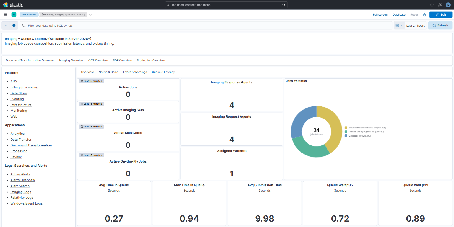
The live-status band summarizes current imaging activity. The active-job tiles count distinct jobs, by job type, that reported job activity in the rolling 15-minute window described above. Job activity means the job was started, picked up by the request agent, submitted (including batch submission), had its population table created or updated, or completed. The tiles show recent activity, not a live count of running jobs: a job that completed a few minutes ago still counts, and a long-running job that reported none of these events in the last 15 minutes does not. The agent tiles show available-agent counts, and the worker tile shows the latest worker-server count:

• Active Jobs - Distinct imaging jobs with job activity in the last 15 minutes, across all job types (imaging sets, retried imaging sets, mass imaging, and on-the-fly).
• Active Imaging Sets - Distinct imaging-set jobs (including retried imaging sets) with job activity in the last 15 minutes.
• Active Mass Jobs - Distinct mass-imaging jobs with job activity in the last 15 minutes.
• Active On-the-Fly Jobs - Distinct on-the-fly imaging jobs (documents imaged individually, on demand) with job activity in the last 15 minutes.
• Imaging Response Agents - Current number of available imaging response agents. This is a count of enabled and available response agents, not threads or messages.
• Imaging Request Agents - Current number of available imaging request agents. Like the response-agent tile, it counts enabled and available request agents, not active threads.
• Assigned Workers - Total number of worker servers in the environment, from the most recent health-check reading. The count includes every worker server, whether or not it is currently active. To check whether a worker is active and accepting work, use the Worker Monitoring tab in Relativity.
• Jobs by Status - A donut showing the current mix of imaging job statuses. Picked Up by Agent (PickedUpByAgent) and Submitted to Invariant (SubmittedToInvariant) are shown with friendly names; other statuses, such as Created, CancelRequested, and Invalid, appear with their raw code. The number in the center, labeled job statuses, is the sum of the slices. For status meanings, see the Job Results Status reference on Imaging Overview.

How to read it: The agent tiles report how many imaging response and request agents are available to pick up work; the Jobs by Status donut shifts toward whichever stage dominates (for example, many jobs Picked Up by Agent during heavy processing). Use this band first to confirm imaging is actively running and that agent and worker capacity is available before investigating the latency panels below.

Reading the screenshot: The screenshot uses a Last 24 hours time range. No jobs reported activity in the last 15 minutes, so all four active-job tiles show 0. Four imaging response agents and four imaging request agents are available. Assigned Workers shows 1, the environment's single worker server. The Jobs by Status donut honors the 24-hour range and is split across Submitted to Invariant (14), Picked Up by Agent (10), and Created (10). Each job is counted once for every status it reported in the selected range, so the total can be higher than the number of jobs. Here, the total of 34 job statuses in the center corresponds to 14 jobs. An idle active-job band with agents available is normal between workloads. However, if jobs stay queued, check the worker servers in Relativity's Worker Monitoring tab, because Assigned Workers counts a worker server even when it is inactive and not accepting work.

Troubleshooting with this band: If the latency panels show rising queue-wait times, check this band for signs that work is not being drained - Assigned Workers at 0 (no worker servers in the environment), or the agent tiles showing 0 available agents while a backlog builds (no imaging agents are enabled to pick up and process the queue). If Active Jobs is high while the queue-wait trend climbs, demand is simply exceeding capacity; if Active Jobs is low but queue wait is still high, the bottleneck is more likely a downstream stage (submission, service bus, or population table) covered in the sections below. For the upstream job composition behind a surge - for example a burst of mass imaging or retries - see the Job Queue Composition donut on the Imaging Overview dashboard.

Queue Latency

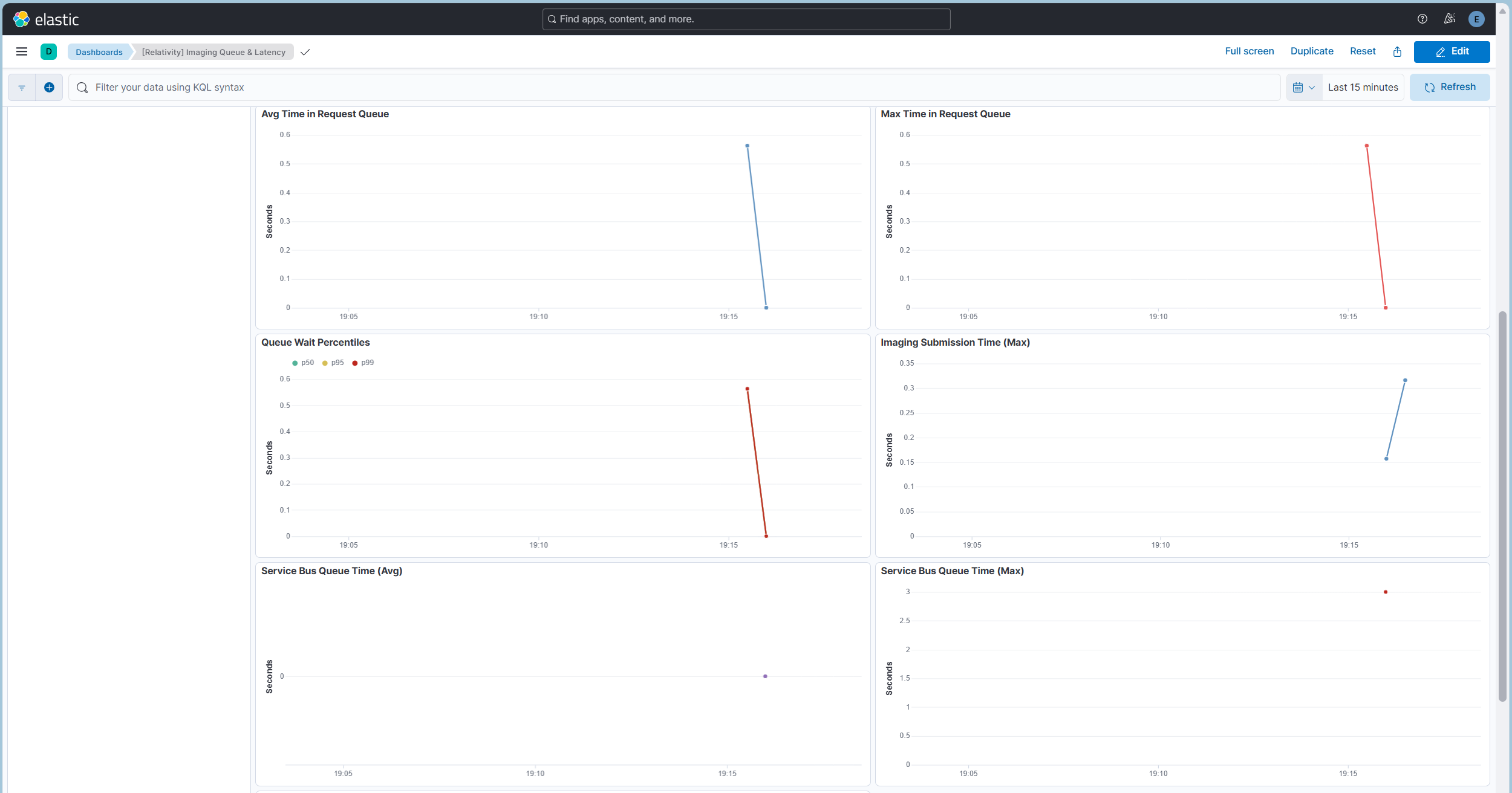
These tiles and trends measure how long imaging jobs wait in the request queue before an agent picks them up - the time between job creation and agent pickup. Latency values are shown in seconds, with trailing zeros trimmed on the axes.

• Avg Time in Queue / Max Time in Queue (tiles) - Average and maximum queue-wait time for the selected range.
• Queue Wait p95 / Queue Wait p99 (tiles) - 95th and 99th percentile queue-wait times, to surface tail latency that an average hides.
• Avg Time in Request Queue / Max Time in Request Queue (trend lines) - The same average and maximum queue wait plotted over time.
• Queue Wait Percentiles (trend line) - A multi-series line showing p50, p95, and p99 queue-wait over time, so tail latency can be tracked alongside the median.

How percentiles work: A percentile describes how the individual queue-wait times are distributed, rather than collapsing them into a single average. For example, p95 = 2s means 95% of jobs waited less than 2 seconds and only the slowest 5% waited longer; p99 isolates the slowest 1%, and p50 is the median - half the jobs waited less than this value. Kibana computes the percentiles across every qualifying job in the selected time range, so widening or narrowing the time picker changes which jobs are included. Because an average is pulled up by a few very slow jobs, comparing the average with p95/p99 is the quickest way to tell a broad slowdown (the whole distribution shifts) from a handful of outliers (only the top percentiles rise).

Hover over a trend chart to see the value for that time bucket; empty buckets show "No data".

How to read it: Read the tiles first for a quick verdict - a low Avg Time in Queue with p95/p99 close to the average means jobs are picked up promptly and consistently; a large gap between the average and p99 means a few jobs wait much longer than typical (tail latency). Then use the Avg / Max Time in Request Queue and Queue Wait Percentiles trend lines to see whether queue wait is steady, trending up (an emerging backlog), or spiking at specific times.

Reading the screenshots: The latency tiles in the Live Status screenshot cover the last 24 hours. Avg Time in Queue is 0.27 s, Queue Wait p95 is 0.72 s, Queue Wait p99 is 0.89 s, and Max Time in Queue is 0.94 s. Every job was picked up in under a second, and 95% within about 0.7 seconds. The average, p95, p99, and maximum are close together, so there is no meaningful tail and no backlog was forming. The queue-wait trend charts above use a Last 15 minutes range and show one short burst of activity at about 19:16: queue wait briefly reached about 0.56 s and then returned to 0. This brief rise-and-return is the expected healthy pattern. A backlog would instead show a line that keeps climbing or stays elevated across buckets.

Troubleshooting with these panels: A sustained rise in Avg Time in Queue (not just an isolated max spike) is the earliest sign of a forming backlog - jobs are arriving faster than agents can pick them up. When you see it, check the Live Status band for a worker shortfall or no available agents (the agent tiles at zero despite a backlog), and confirm whether Active Jobs rose at the same time (a genuine demand surge) or stayed flat (a pickup bottleneck despite low demand). Use the percentile trend to distinguish a broad slowdown (p50 rises) from a few slow outliers (only p95/p99 rise). If queue wait is healthy but jobs still complete slowly, the delay is downstream - continue to the submission, service-bus, and population-table panels below.

Related sections: Compare these queue-wait panels with the Submission, Service Bus & Population Table Latency panels below to localize where time is spent, and with the Live Status band above to relate queue wait to current capacity. On the Imaging Overview dashboard, the Jobs Submitted / Jobs Picked Up by Request Agent / Jobs Completed tiles corroborate whether the queue is draining.

Submission, Service Bus & Population Table Latency

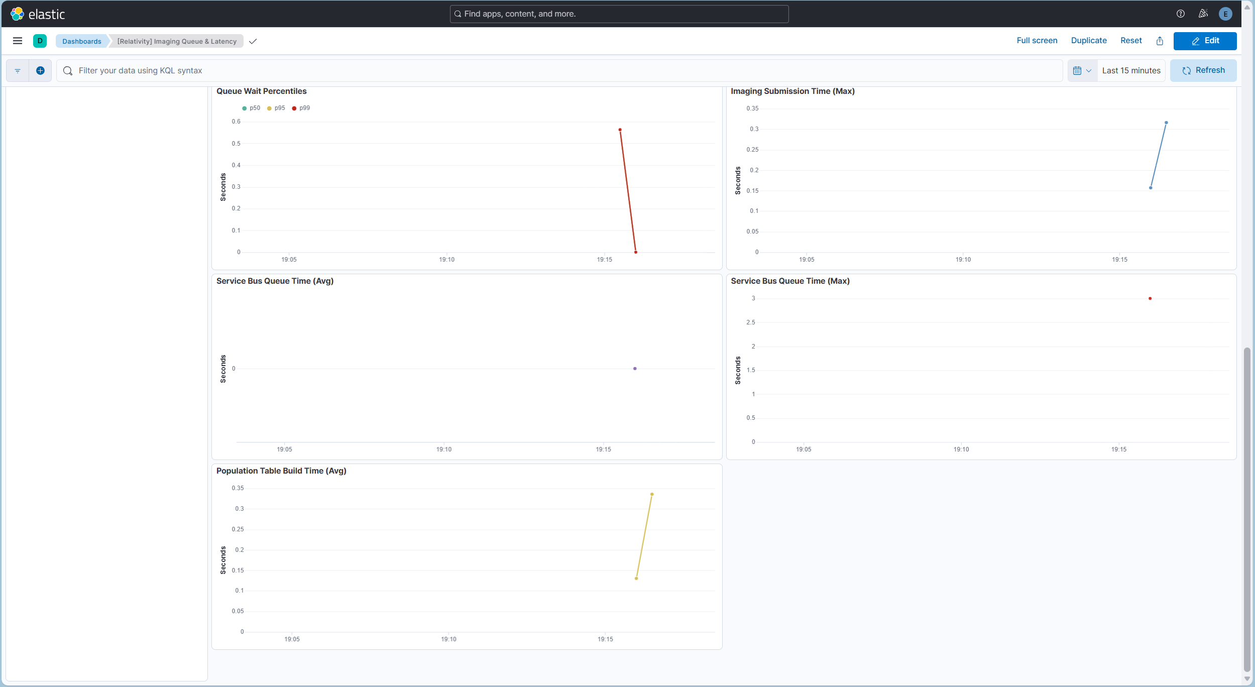
These panels measure other timing stages of the imaging pipeline. The Avg Submission Time tile appears in the Live Status screenshot and the Imaging Submission Time (Max) trend in the Queue Latency screenshot; the Service Bus and Population Table trends are shown here. All values are in seconds and honor the dashboard time range:

• Avg Submission Time (tile) - Average time to submit a job for imaging. Submission time is the time it takes an imaging job to submit all of its documents to Invariant, measured from when the Imaging Request Agent picked up the job.
• Imaging Submission Time (Max) (trend line) - Maximum submission time over time.
• Service Bus Queue Time (Avg) (trend line) - Average time messages spend in the service-bus queue, reported from service-bus queue-status events.
• Service Bus Queue Time (Max) (trend line) - Maximum service-bus queue time.
• Population Table Build Time (Avg) (trend line) - Average time to create or update the population table, the database step imaging performs as part of processing.

How the service-bus stage works: Imaging passes work between its request and response agents and the Invariant conversion workers over a message bus. After a document is imaged, its completion (response) message waits briefly in the service-bus queue before the response agent picks it up and records the result; that per-document wait is captured for every document in the job. The Service Bus Queue Time (Avg / Max) trends plot the average and maximum of those per-document waits over time, so a sustained rise in both - rather than a lone max spike - indicates the messaging layer is backing up rather than any single slow message.

How the population table works: As part of running a job, imaging creates - or, on later passes, updates - a per-job working table in the workspace database (the population table) that enumerates the documents to be imaged and tracks each document's imaging status and per-document results. Population Table Build Time (Avg) measures how long that create/update step takes. Because it is a database operation, a rise points to database contention during the population step itself rather than to the imaging conversion that follows.

How to read it: These stages sit around the core queue wait, so use them to localize where latency originates. A spike in Submission Time points to slow job submission to Invariant; a spike in Service Bus Queue Time points to messaging-layer backpressure; a spike in Population Table Build Time points to a slow database step. When queue-wait latency rises, compare these trends to see which stage moved at the same time. The screenshots use a Last 15 minutes range, and the same short burst at about 19:16 appears in each one. Imaging Submission Time (Max) is about 0.3 s, Service Bus Queue Time is 0 s on average with a 3 s maximum, and Population Table Build Time ranges from about 0.13 s to 0.34 s. These are brief, low values from a healthy pipeline. The 24-hour Avg Submission Time tile in the Live Status screenshot (9.98 s) is higher because it averages over a full day of jobs, including larger ones. A brief isolated spike in a max line usually reflects a single outlier job rather than a systemic slowdown.

Troubleshooting with these panels: Line up the time axes of these trends with the Avg Time in Request Queue, Max Time in Request Queue, and Queue Wait Percentiles trends in the section above. If overall job completion slows but queue wait stays flat, the stage whose line moves here is the likely cause: sustained high Submission Time suggests Invariant or document-submission pressure; a rising Service Bus Queue Time (average and max climbing together) suggests the messaging layer is backing up rather than a single slow message; a rising Population Table Build Time suggests database contention during population-table creation. Prefer a sustained shift over a lone max spike before concluding a stage is at fault.

Related sections: These stages complement the queue-wait panels above (where jobs wait before pickup) and the Live Status band (current capacity). For the error and warning side of imaging health - which can accompany or follow a latency event - see the Errors & Warnings dashboard.

Investigating Queue and Latency Issues

The panels are arranged top-to-bottom to support a consistent investigation flow: confirm activity and capacity, read the queue-wait verdict, then localize the responsible stage.

1. Confirm imaging is running and has capacity. Start with the Live Status band. Verify Active Jobs is non-zero (over the last 15 minutes), that Imaging Response Agents and Imaging Request Agents show available agents while jobs run, that Assigned Workers is non-zero, and that the Jobs by Status donut shows jobs progressing (for example, moving into Picked Up by Agent and Submitted to Invariant). If there are no workers, or jobs are stuck in an early status while the agent tiles stay at zero, that is the first thing to address. If worker servers are present but jobs still do not progress, check in Relativity's Worker Monitoring tab that the workers are active.

2. Diagnose a queue backlog. Set the time picker to the window in question and read the Avg Time in Queue and Max Time in Queue tiles. If the average is rising across the Avg Time in Request Queue trend, a backlog is forming. Check whether Active Jobs rose at the same time (demand exceeding capacity) or stayed flat (a pickup bottleneck despite normal demand), and cross-check worker availability and whether imaging agents are available in the Live Status band.

3. Catch tail latency the average hides. Compare Queue Wait p95 and Queue Wait p99 with Avg Time in Queue. A large gap means a minority of jobs wait far longer than typical. Use the Queue Wait Percentiles trend to tell a broad slowdown (p50 rises with p95/p99) from a few slow outliers (only p95/p99 rise), and note when the tail widened.

4. Localize the slow stage. If jobs complete slowly but queue wait is flat, align the time axes of Imaging Submission Time (Max), Service Bus Queue Time (Avg/Max), and Population Table Build Time (Avg) with the queue-wait trends. The stage whose line moves at the same time points to the layer to examine - submission to Invariant, the service-bus messaging layer, or the population-table database step. Prefer a sustained shift over a single max spike.

5. Relate latency to composition and outcomes. For the job composition behind a surge (a burst of mass imaging or retries) and for throughput and success/error outcomes, move to the Imaging Overview dashboard; for the specific errors or warnings accompanying a latency event, use the Errors & Warnings dashboard.

Use Cases

Use Case	Description
Confirm imaging is running	Use the Live Status tiles to verify recent job activity, that imaging agents are available, and that worker servers are present.
Check current workload mix	Use Jobs by Status to see the current distribution of imaging job statuses.
Detect queue backlog	Use Avg/Max Time in Queue and the queue trend lines to spot rising queue-wait times before they become a backlog.
Investigate tail latency	Use Queue Wait p95/p99 and the Queue Wait Percentiles trend to catch slow outliers the average hides.
Diagnose submission delays	Use Avg Submission Time and Imaging Submission Time (Max) to find slow job submissions.
Monitor infrastructure timing	Use the Service Bus Queue Time and Population Table Build Time trends to correlate latency with messaging or database stages.
Localize a latency stage	Align the submission, service-bus, and population-table trends with the queue-wait trends to identify which stage moved when job completion slowed.
Validate capacity	Compare Active Jobs against Assigned Workers and available imaging agents to judge whether processing is keeping up with demand.

Associated Alerts

No imaging-specific Environment Watch alerts are currently associated with this dashboard. This section will be updated as imaging alerts are published.